Microphone magnitude frequency response correction

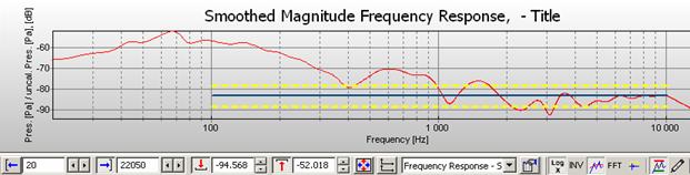
If you want to plot the frequency response as shown in the figure below, you can apply a correction for the magnitude frequency response of your microphone. Note that this compensation will only apply to this magnitude frequency response plot type (it can also be selected for the waterfall plot type, but not any of the other plot types). So for many applications you can skip this part.

The data for your microphone needs to be in a file containing the frequencies as first row and level as second row. You can write comments in the upper lines. An example of such a microphone compensation file is shown below using comma as separator, you may also use tab as separator.

"Transfer Function Mag - dB volts/volts”

      "Hz"      "Data"

  13.81928,   5.60

  50.67069,   5.60

  198.0763,   5.07

  999.5946,   4.52

  3,150.796,   4.31

  10,000.55,   2.88

  15,998.12,   1.58

   20,001.1,  -0.78

  24,999.08,  -5.81

WinMLS will do a spline interpolation of the data so that a continuous spectrum compensation will be made.

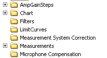
Save such a file with the extension ‘.txt’ under the WinMLS subfolder named Microphone Compensation shown at the bottom in the figure below.

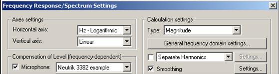
To turn on the microphone compensation, go to Plot->Plot Type Settings->Frequency Response/Spectrum.... This will open the dialog box shown below.

Now make sure  is checked. Then select the microphone compensation file, in the figure above we have selected the file named ‘Neutrik 3382 example.txt’ . It is also possible to correct for multiple microphones in case you are doing multi-channel measurements.