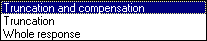
Integration options
After filtering, backwards integration of the impulse response to form a decay curve, or Schroeder curve, is done as further preparation to the parameter calculations. If h(t) is the filtered impulse response, the decay curve is:
(1)
This provides a monotonically falling decay. The curve is usually normalized to start at 0dB. In practice the impulse response record is finite, and the integration becomes finite as well:
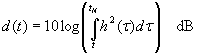
(2)
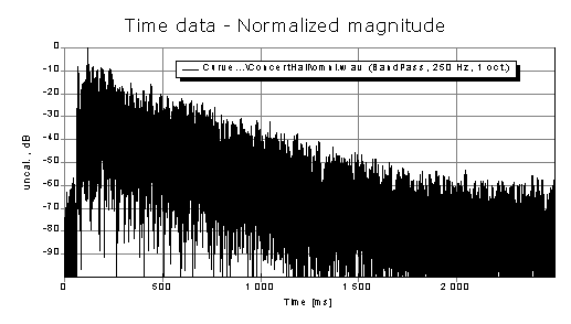
Also, a measured response tends to contain some noise. Due to the phase randomizing property of the MLS deconvolution, additive noise of any kind in the measurement will give rise to a stationary noise floor, see the example below. This is advantageous as a combined noise-decay analysis of the filtered impulse response record can reveal the location of the cross-point between the response and the stationary noise floor, the response can be truncated at or above this point to lessen the influence of the noise on the results, and finally the truncated energy can be estimated and taken into consideration.
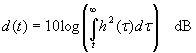
If compensation for truncated energy is incorporated, and the estimated correction is denoted C, the decay curve is:
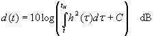
(3)
The integration options are shown and explained below.