How to plot spectrum in octave or third-octave bands?

The easiest way is to load the setup called QuasiRealTimeAnalyzer. Below it is described more in detail how it can be done without loading the setup. This is not intended to be used for transfer function measurements, since it will give a 3 dB/octave bias because of the integration explained below.

The energy or power can be plotted in octave or third-octave bands if Frequency response/Spectrum is selected as plot type. In Plot->General Frequency Domain Settings... select the scope mode to one of the below.

What you choose depends on if the signal you are analyzing is stationary or transient.

Click F5 to display the plot settings dialog box. Make sure that Use Smoothing (or integration) is checked as shown in the figure below. Click on the Settings… button also shown in the figure below.

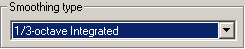
In the new dialog box, select smoothing type as shown below (or select the 1-octave Integrated option).

Click OK to exit the dialog boxes.

An example of 1/3 octave normalized energy is displayed in the figure below.

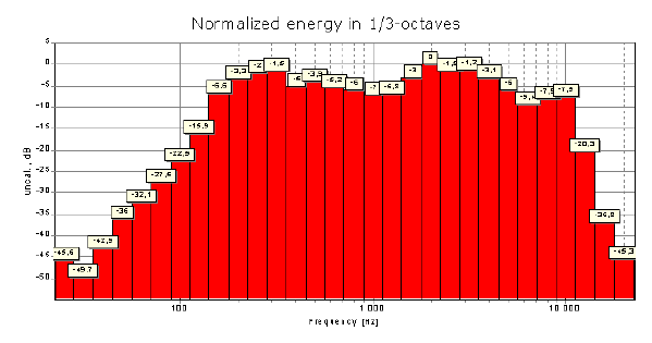
In this figure, we have used curve type Histogram to get the bars (can be set in the bottom of the Plot->Advanced Plot Settings… dialog box). For information about how to display the values for each point, see How to change the curve style (color, type and width)?